Introduction to Partial Differential Equation (PDE)

Introduction

PDE can be classified as elliptic, parabolic or hyperbolic. In fluids dynamics, the governing equations contain first and second derivatives in the spatial coordinates and first derivatives only in time. The spatial derivatives often appear nonlinearly while the time derivatives appear linearly. For linear PDE of second-order in two independent variables $x$ and $y$,

$A\frac{\partial^2 u}{\partial x^2} + B\frac{\partial^2 u}{\partial x \partial y} + C\frac{\partial^2 u}{\partial y^2} + D\frac{\partial u}{\partial x} + E\frac{\partial u}{\partial y} + Fu + G =0$

A simple classification is as follows.

• If $B^2 - 4AC < 0$: elliptic PDE
• If $B^2 - 4AC = 0$: parabolic PDE
• If $B^2 - 4AC > 0$: hyperbolic PDE

In many cases, $B=0$. Under this condition,

• If $AC > 0$: elliptic PDE
• If $AC = 0$: parabolic PDE
• If $AC < 0$: hyperbolic PDE

Why? Lets see the characteristics for a single first-order PDE (*):

$A\frac{\partial u}{\partial t} + B\frac{\partial u}{\partial x} = C$

The characteristic direction is defined by

$\frac{d x}{d t} = \frac{B}{A}$

in which the relation between $x$ and $t$ can be built (See $C$=0). It is known that the definition of the total differential is:

$du = \frac{\partial u}{\partial t}dt + \frac{\partial u}{\partial x}dx$

$\frac{du}{dt} = \frac{\partial u}{\partial t} + \frac{\partial u}{\partial x} \frac{dx}{dt}$

$A \frac{du}{dt} = A \frac{\partial u}{\partial t} + A \frac{\partial u}{\partial x} \frac{dx}{dt}$

If we can find the solution of $A\frac{du}{dt}= C$ and $\frac{dx}{dt}=\frac{B}{A}$, the problem (*) can be solved. Therefore, the equations by $\frac{dx}{dt}=\frac{B}{A}$ plus $\frac{du}{dt}=\frac{C}{A}$ give the characteristic curve of the PDE.

For a two-order PDE with two independent variables $x$ and $y$:

$A\frac{\partial^2 u}{\partial x^2} + B\frac{\partial^2 u}{\partial x \partial y} + C\frac{\partial^2 u}{\partial y^2} + H = 0$

where $H$ contains all the first derivative terms and constant terms. The total differential can be written as:

$du = \frac{\partial u}{\partial x}dx + \frac{\partial u}{\partial y}dy$

$\frac{du}{dx} = u_x + u_y y'$

The characteristic equation is given as:

$A {y'}^2 - By' + C = 0$

The solutions $\frac{B\pm \sqrt{B^2 - 4AC}}{2A}$ are the characteristic curves ($A\neq 0$).

• If $B^2 - 4AC > 0$, two real characteristics exist, lead to a hyperbolic PDE.
• If $B^2 - 4AC = 0$, only one real characteristic exists, lead to a parabolic PDE.
• If $B^2 - 4AC < 0$: two complex characteristics exist, lead to an elliptic PDE.

By the way, using characteristics is a dimensionality reduction. A coordinate transformation does not change the type of PDE. It can be proved that $B_2^2-4A_2C_2 = J^2(B_1^2-4A_1C_1)$. $J$ is the Jacobian of the transform. For a general case, a two-order PDE with $N$ independent variables:

$\sum_{i=1}^N \sum_{j=1}^N a_{ij} \frac{\partial^2 u}{\partial x_i \partial x_j} + H = 0$

Let $\lambda$ be the eigenvalues of the coefficient matrix with elements $a_{ij}$.

• If all $\lambda$ are non-zero and all but one are the same sign, it leads to a hyperbolic PDE.
• If any of $\lambda$ is zero, it leads to a parabolic PDE.
• If all $\lambda$ are non-zero and of the same sign, it is an elliptic PDE.

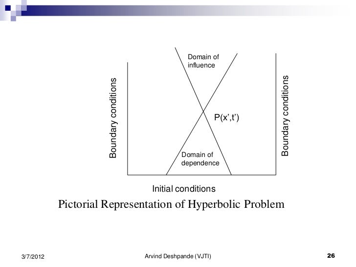
Hyperbolic PDE

A simple example is the 1-D wave equation.

$\frac{\partial^2 u}{\partial t^2} - c^2\frac{\partial^2 u}{\partial x^2} = 0$

where the characteristic directions are give by $dx/dt=\pm c$. $c$ is the wave speed.

The equation has the property that, if $u$ and $\frac{\partial u}{\partial t}$ are arbitrarily specified initial data on the line $t = 0$ (with sufficient smoothness properties), then there exists a solution for all time $t$. The solutions of hyperbolic equations are “wave-like”. Disturbances of the initial or boundary conditions have a finite propagation speed. On the contrary, a perturbation of an elliptic or parabolic equation is felt at once by essentially all points in the field. No dissipative mechanism exists for hyperbolic equations. If the initial or boundary data contain discontinuities they will be transmitted into the interior along characteristics without attenuation.

Parabolic PDE

The unsteady Navier-Stokes equations are parabolic. A simple example is the 1-D heat conduction equation (diffusion equation).

$\frac{\partial u}{\partial t} - \alpha \frac{\partial^2 u}{\partial x^2} = 0$

where $\alpha$ is the thermal diffusivity. The heat conduction signal is felt immediately throughout the system.

The parabolic equation has a single characteristic direction defined by $dx/dt=\infty$($dt/dx=0$). Following the characteristics would never advance the solution in time. The solutions of hyperbolic equations are dissipative in space while marching forward in time. It means a disturbance introduced at $P$ can influence anywhere in the computational domain for $t>t_i$ with an attenuated magnitude. Even if the initial conditions include a discontinuity, the solution in the interior will always be continuous.

Note that the parabolic PDEs in two or three dimensions are elliptic for the steady state ($\frac{\partial u}{\partial t} = 0$). The 2-D or 3-D heat conduction equation is also paraolic. The 2-D or 3-D steady state heat conduction equation are elliptic.

Elliptic PDE

For fluid dynamics, as mentioned before, elliptic PDE are associated with steady-state problems. A simple example is the Laplace’s equation.

$\frac{\partial^2 \phi}{\partial x^2} + \frac{\partial^2 \phi}{\partial y^2} = 0$

For the second order elliptic PDEs, the maximum principle says, both the maximum and minimum values of $\phi$ must occur on the boundary, except the case when $\phi=$constant.

Traditional solution methods