机器学习笔记（4）贝耶斯分类

Introduction

Here is a not so short note (Rolling Update) for machine learning and artificial intelligience. Main concepts and some references are presented. This note is based on Wikipedia, Andrew Ng’s Lecture Notes CS229 of Standford, Machine Learning course of SJTU IEEE-yangyang, and Machine Learning Crash Course of Google.

Bayesian estimation

If you flip a coin, what’s the probability it will fall with the head up? To solve this problem, you may flip the coin many times. You will get the data:

$X=\{X_i\}^n_{i=1}, X_i \in {H,T}$

where $H$ means Head and $T$ means Tail. The probabilityshould be:

$P(Head) = \theta, P(Tail) = 1 - \theta$

If you flip the coin 100 times, with 57 heads and 43 tails, the probability of $P (Head)$ should be 57/100. Because the flips are i.i.d., which means:

• Independent events
• Identically distributed according to Bernoulli distribution ($n=1$ means BErnoulli distribution)

Maximum likelihood estimation

The aim of the maximum likelihood estimation is to choose $\theta$ that maximizes the probability of observed data. MLE of probability of head can be calculated based on i.i.d. as below:

$\hat{\theta}_{MLE} = \arg \max \limits_{\theta} P(X \mid \theta)$

$= \arg \max \limits_{\theta} \prod_{i=1}^n P(X_i \mid \theta)$

$= \arg \max \limits_{\theta} \prod_{i:X_i=H}^{\alpha_H} \theta \prod_{i:X_i=T}^{\alpha_T} (1-\theta)$

$= \arg \max \limits_{\theta} \theta^{\alpha_H} (1-\theta)^{\alpha_T}$

Let $J(\theta)=\theta^{\alpha_H}(1-\theta)^{\alpha_T}$. It is easy to find the $\theta$ that maximizes the probability of observed data:

$\frac{\partial J(\theta)}{\partial \theta} \Big\vert_{\theta=\hat{\theta}_{MLE}} = 0$

Thus the MLE of probability of head is:

$\hat{\theta}_{MLE} = \frac{\alpha_H}{\alpha_H+\alpha_T}$

Prior and posterior

If you flip a coin 5 times, it is possible that 5 heads are obtained. In this case, the probability of head will be 1.0 if you use the maximum likelihood estimation. However, it is crazy to consider that the result of fliping a coin is always head. Thus, we need to use prior probability to adjust the probability calculation.

A prior probability distribution of an uncertain quantity is the probability distribution that would express one’s beliefs about this quantity before some evidence is taken into account. A prior can be determined from past information such as previous experiments, or according to some principle such as Jeffreys prior.

A posterior probability distribution of an unknow quantity is the probability distribution treated as the conditional probability that is assigned after the relevant evidence or background is taken into account. In contrasts with the likelihood function $P(X \mid \theta)$, the posterior probability is given as:

$P(\theta \mid X) = \frac{P(X \mid \theta)P(\theta)}{P(X)}$

where $P(\theta)$ is probability density function (pdf) of the prior probability.

Conjugate prior

In Bayesian probability theory, if the posterior distributions $P(\theta \mid X)$ are in the same probability distribution family as the prior probability distribution $P(\theta)$, the prior and posterior are then called conjugate distributions, and the prior is called a conjugate prior for the likelihood function. When a family of conjugate priors exists, choosing a prior from that family simplifies posterior form.

An example of the conjugate prior: In the problem of coin flipping,

• Likelihood is ~ binomial distribution:

$P(X \mid \theta) = \left( \begin{matrix} n \\ \alpha_H \end{matrix} \right) \theta^{\alpha_H} (1-\theta)^{\alpha_T}$

$= \frac{n!}{\alpha_H! (n-\alpha_H)!} \theta^{\alpha_H} (1-\theta)^{\alpha_T}$

It means in $n$ independent flipping trial, the probability of occurring $\alpha_H$ heads belongs to binomial distribution, with the probability of head is $\theta$ for every flipping.

• Prior is assumed as Beta distribution:

$P(\theta) = \frac{\theta^{\beta_H-1} (1-\theta)^{\beta_T-1}}{B(\beta_H,\beta_T)} \sim Beta(\beta_H,\beta_T)$

where $B(\beta_H,\beta_T)=\frac{\Gamma(\beta_H) \Gamma(\beta_T)}{\Gamma(\beta_H+\beta_T)}$, $\Gamma(z)$ is the gamma function as an extension of the factorial function, $\Gamma(z) = \int_0^{\infty} x^{z-1}e^{-x} dx$, and $\Gamma(n) = (n-1)!$, if $n$ is a positive integer.

• Posterior is also Beta distribution:

$P(\theta \mid X) \sim Beta(\beta_H + \alpha_H,\beta_T + \alpha_T)$

For binomial distribution, the conjugate prior is Beta distribution. The pdf of Beta distribution got more concentrated as values of $\beta_H$ and $\beta_T$ increased. As more samples are obtained, $\beta_H + \alpha_H >> \beta_H$, the effect of prior will be “washed out”.

Another example of the conjugate prior: In the problem of rolling a dice, there are $k=6$ outcomes.

• Likelihood is ~ multinomial ($\theta={\theta_1,\theta_2,...,\theta_k}$)

$P(X \mid \theta) = \frac{n!}{\alpha_1!\alpha_2!...\alpha_k!} \prod_{i=1}^k \theta_i^{\alpha_i}$

The multinomial distribution is a generalization of the binomial distribution. In $n$ independent rolling test, the probability of occurring $\alpha={\alpha_1,\alpha_2,...,\alpha_k}$ times of the dice number $\alpha={X_1,X_2,...,X_k}$ belongs to multinomial distribution, with the probability of $X_k$ is $\theta_k$ for every rolling. The sum of $\theta_k$ is 1 and the sum of $\alpha_k$ is $n$.

• Prior is assumed as Dirichlet distribution:

$P(\theta) = \frac{\prod_{i=1}^k \theta_i^{\beta_i -1}}{B(\beta_1,\beta_2,...,\beta_k)} \sim Dir(\beta_1,\beta_2,...,\beta_k)$

• Posterior is also Dirichlet distribution:

$P(\theta \mid X) \sim Dir(\beta_1+\alpha_1,\beta_2+\alpha_2,...,\beta_k+\alpha_k)$

For multinomial, the conjugate prior is Dirichlet distribution.

MLE compared with MAP: maximum a posterior estimation

• MLE: to choose $\theta$ that maximizes the likelihood probability (the probability of observed data) P(X \mid \theta).
• MAP: to choose $\theta$ that maximizes the posterior probability P(\theta \mid X).

$\hat{\theta}_{MAP} = \arg \max \limits_{\theta} P(\theta \mid X)$

$= \arg \max \limits_{\theta} P(X \mid \theta)P(\theta)$

In the problem of flipping trial, the maximum a posterior estimation of probability of head is Beta distribution:

$P(\theta \mid X) \sim Beta(\beta_H+\alpha_H,\beta_T+\alpha_T)$

MLE vs MAP:

$\hat{\theta}_{MLE} = \frac{\alpha_H}{\alpha_H+\alpha_T}$

$\hat{\theta}_{MAP} = \frac{\alpha_H + \beta_H - 1}{\beta_H+\alpha_H+\beta_T+\alpha_T-2}$

For small sample size, the prior is important. For infinite $n$, prior will be useless. Therefore, when $\beta_H=\beta_T=1$, MAP will be same as MLE.

We use Gaussian distribution for a continuous variable $x$ which is i.i.d. The central limit theorem (CLT) establishes that, in most situations, when independent random variables are added, their properly normalized sum tends toward a normal distribution

The pdf is $N(\mu,\sigma^2)$:

$P(x \mid \mu,\sigma) = \frac{1}{\sigma \sqrt{2\pi}} e^{\frac{-(x-\mu)^2}{2\sigma^2}}$

where $\mu$ is the mean and $\sigma^2$ is the variance.

MLE probability for Gaussian distribution:

$\hat{\theta}_{MLE} = \arg \max \limits_{\theta} P(X \mid \theta)$

$= \arg \max \limits_{\theta} \prod_{i=1}^n P(X_i \mid \theta)$

MLE for Gaussian mean and variance:

$\mu_{MLE} = \frac{1}{n} \sum_{i=1}^n x_i$

$\sigma_{MLE}^2 = \frac{1}{n} \sum_{i=1}^n (x_i - \hat{\mu})^2$

Here we use average value to estimate $\mu$, which is not a true parameter. The estimation of $\sigma$ is under-estimated thus MLE for the variance of a Gaussian is biased. Because the average of ${x_1,x_2,...,x_n}$ is used as $\hat{\mu}$, the true mean is not equal to the average of samples. If we use the average of samples to estimate the average of total, there will be a bias. For a unbiased variance estimator:

$\sigma_{unbiased}^2 = \frac{1}{n-1} \sum_{i=1}^n (x_i - \hat{\mu})^2$

Because only $n-1$ $x_i$ is independent with the average of samples. The $n^{th}$ $x_i$ can be obtained by the average and other $n-1$ values, which includes no additional information.

If we use different samples, the mean is also different. The prior for mean is also Gaussian distribution:

$P(\mu \mid \eta,\lambda) = \frac{1}{\lambda\sqrt{2\pi}}e^{\frac{-(\mu-\eta)^2}{2\lambda^2}}$

The conjugate prior for mean is Gaussian distribution and for variance is Wishart distribution.

Bayes classifier

Bayes Optimal Classifier

Bayes optimal classifier is a kind of ensemble learning. In Bayesian learning, the primary question is: What is the most probable hypothesis give data? If we have:

• X: Features
• Y: Target classes
  How to decide which class $y$ is for a new sample with feature $x$? ($x\in X$ and $y\in Y$)

The Bayes rule is:

$P(Y=y \mid X=x) = \frac{P(X=x \mid Y=y)P(Y=y)}{P(X=x)}$

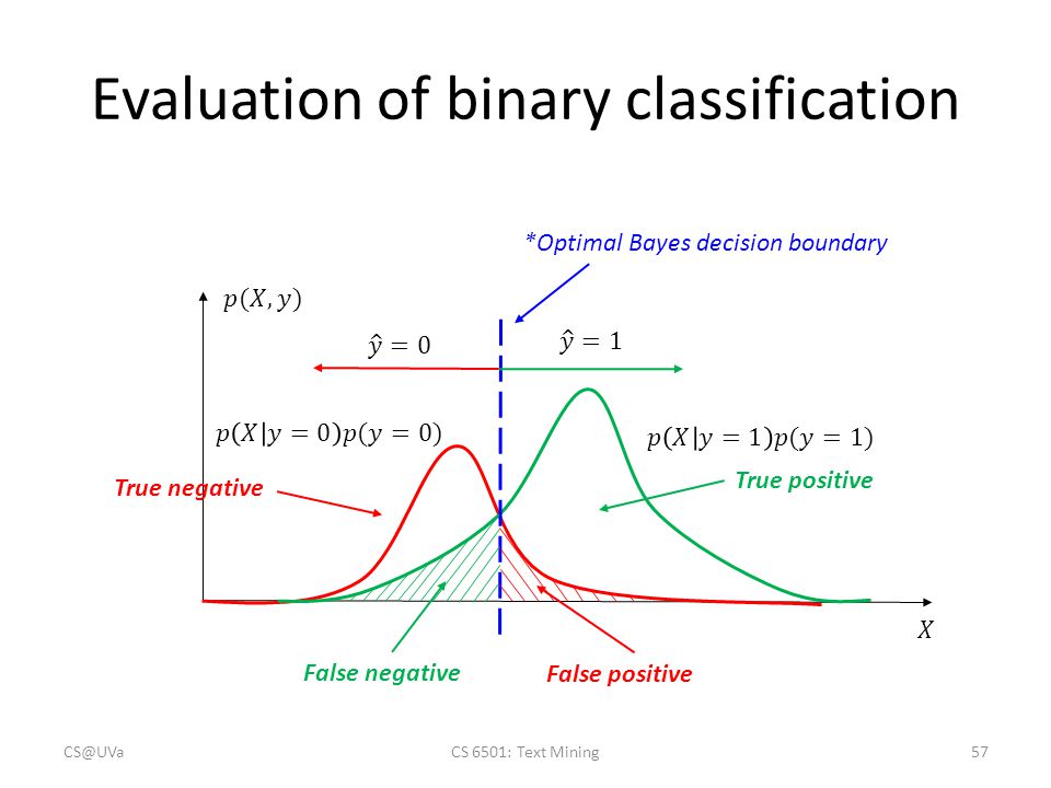
According to the Bayes decision rule, we need to minimize the conditional risk of making a wrong classification of a sample. Becasue $R(y \mid x)=1-P(y \mid x)$, the Bayes optimal classifier can be written as:

$h^*(x) = \arg \max \limits_{Y=y} P(Y=y \mid X=x)$

As the denominator $P(X=x)$ is fixed for call cases, the maximum can be derived as:

$h^*(x) = \arg \max \limits_{Y=y} P(X=x \mid Y=y)P(Y=y)$

• $P(X=x \mid Y=y)$ is the class conditional density (likelihood)
• $P(Y=y)$ is the class prior

A binary classification and the optimal Bayes decision boundary is shown as follows.

Conditional independence

Given Z, X is conditionally independent of Y means:

$P(X,Y \mid Z) = P(X \mid Z)P(Y \mid Z)$

e.g. If the alarm in your house is active (Z), your neighbor Mary will call the police (X) or another neighbor John will call the police (Y). It is assumed that they do not communicate for each other. In this case, Mary’s calling and John’s calling are conditionally independent. It also means whether Mary’s calling the police is irrelated to John’s calling:

$P(X \mid Y,Z) = P(X \mid Z)$

Note: Independence $\nLeftrightarrow$ Conditionally Independence
X is conditionally independent of Y with a given Z, does not mean that, X is independent of Y. e.g. It is unknown whether Mary’s calling is independent of John’s calling. They can call the police for other cases other than the alarm in your house. On the contrary, X is independent of Y, does not result to, X is conditionally independent of Y with a given Z. e.g.

• X: rolling a dice, the number is 3.
• Y: rolling a dice, the number is 2.
• Z: rolling a dice two times, the sum of the two numbers is 5.
  In this case, X is not conditionally independent of Y with the given Z.

Naive Bayes (NB)

Naive Bayes Optimal Classifier assumes that the data is conditionally independent on the given class, which makes the computation more feasible.

$P(X_1,...,X_d \mid Y) = \prod_{i=1}^d P(X_i \mid Y)$

where $d$ is the number of features. For each discrete feature, the likelihood is $P(X_i \mid Y)$. If the class prior is $P(Y), the decision rule of Naive Bayes can be:

$h^*_{NB}(x) = \arg \max \limits_{y} P(x_1,x_2,...,x_d \mid y)P(y)$

$= \arg \max \limits_{y} \prod_{i=1}^d P(x_i \mid y)P(y)$

Actually, the features are not conditionally independent, then

$P(X_1,...,X_d \mid Y) \neq \prod_{i=1}^d P(X_i \mid Y)$

Nonetheless, Naive Bayes sometimes still performs well even when the assumption of conditionally independence is violated. If the training data is insufficient, e.g., there is no sample for a feature $X_1$ in the class $Y$, the likelihood will be zero. No matter what the values $X_2,...,X_d$ take, the probability keeps zero as:

$P(X_1,...,X_d \mid Y) = 0$

If the features are continuous, we use Gaussian Naive Bayes (GNB) instead. Let $X_i = x$ and $Y=y_k$. The probability is:

$P(x \mid y_k) = \frac{1}{\sigma_{ik}\sqrt{2\pi}} e^{\frac{-(x-\mu_{ik})^2}{2\sigma_{ik}^2}}$

The subscript indicates the mean and variance for each class $k$ and each feature $i$ are different.

Reference

[1] Some common probability distributions
[2] Why use $n-1$ for unbiased variance estimation
[3] Example of NB: Sex classification based on features including height, weight, and foot size